Image Processing

Linear Image Transformations

Computer Graphics Notes have information about types of transformations and homogenous coordinates.

Image Interpolation

Direct interpolation lead to black spots, so instead we use indirect interpolation.

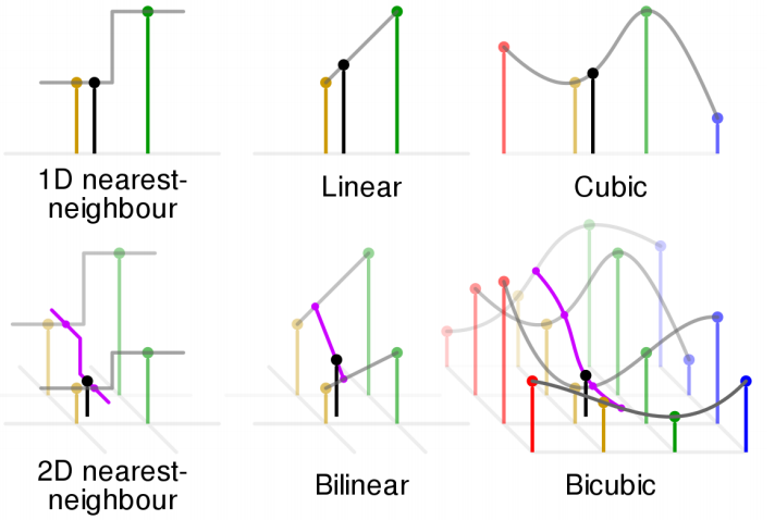
For Bilinear interpolation \(I_{x,y} = \omega_4I_{u,v} + \omega_3I_{u+1,v} + \omega_2I_{u,v+1} + \omega_1I_{u+1,v+1}\)

Cubic interpolation retains grey values but requires 10x more computation than NN and 2x more computation than bilinear interpolation.

Image Filtering

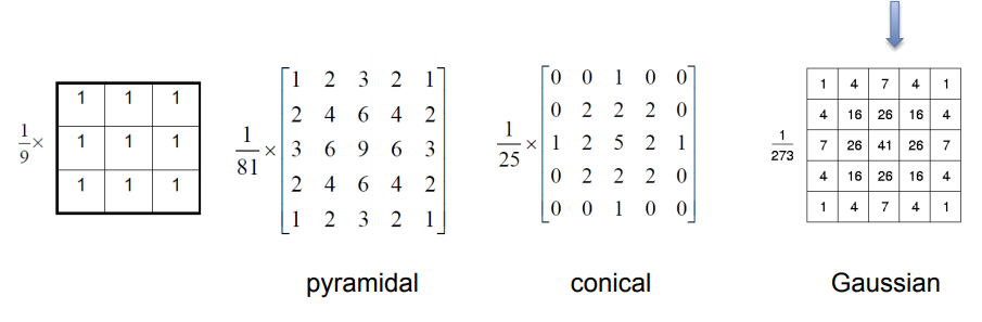
There are two main types of filers - high-pass filters that detect change and low-pass filters that remove noise.

Can either be applied in the frequency domain via a Foruier transform or in the spatial domain via a convolution.

We can modify the pixels in the image either point-wise, locally, or globally.

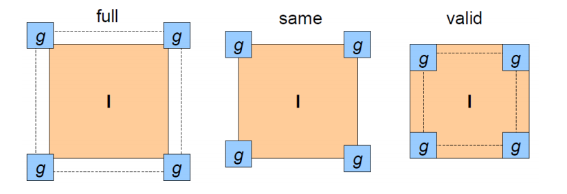
We can handle borders by either clipping, wrapping around, propogating the edge, or reflecting across an edge.

Filtering by Convolution

\(I'(x,y) = \sum_{i=-1}^{1}\sum_{j=-1}^{1}{I(x+i, y+j) \times filter(i,j)}\)

Convolutional filters are commutative, associative, and distributive.

By subtracting the low-pass filter from the source image, we get a high-pass filter.

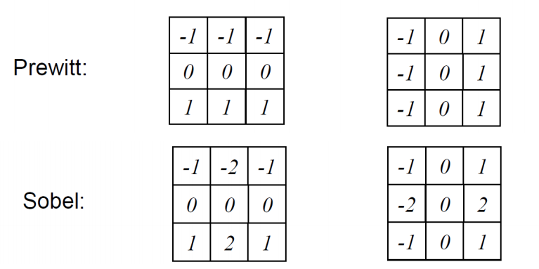
Using Graidents and Laplacians

To improve edge detection, we can take the derivative/2nd derivative of the signal via a convolution using the numerical approximation of the derivative.

Some filters are seperable, which means they can be expressed as the product of two vectors. Since convolutions are associative, this means we can run in \(O(M)\) instead of \(O(M^2)\)

We can sharpend images by applying a high pass filter and then adding this detail back into the image.

Filtering images via convolutions also lets us apply deconvolutions to images, which allow us to extract original images.

However, the convolution matrix is not square so to inverse it we use the Moore-Penrose Pseudoinverse \((A^TA)^{-1}A^T\)

Feature Detection

We can use blob detection to find regions of interest.

Ideally, we want scale invariance so that the scale of key features do not matter.

To do this, we can use edge detection using the Laplacian, or 2nd derivative. When the second derivative crosses 0, we know there is an edge.

However, the max response occurse when the zeros of the laplacian line up with the circle, \(\sigma = r/\sqrt{2}\). If the scale is too large we may not detect images, while if it is too small we may have too much noise.

To get around this, we can convolve the image with the Laplacian at several scales and take the max of the response to find blobs of all sizes.

Affine Covariance

Not all blobs are circular, must deal with affine transformations.

To deal with rotation, we can instead take a histogram of pixel values.

Alternatively, we can compute the average/max of the gradients for each portion of the image, and use this to align the images.

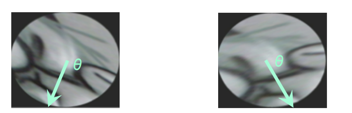
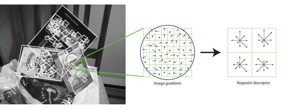
SIFT

SIFT is a histogram of the gradients of the image across small patches.

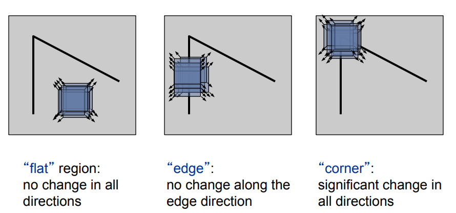
Corners and Interest Points

Humans naturally use corners and other points of interest to aligh ourselves. These points are usually represented by a large change in color, intensity, or texture.

Can be used for image registration, stereo matching, or panorama stitching.

Ideally, we should be able to use the gradient to detect corners.

Harris Corner Detector - \(A_W = \sum_{x \exists W, y \exists W}{w(x,y) \begin{bmatrix} f_x^2 & f_xf_y \\ f_xf_y & f_y^2 \end{bmatrix}}\)

where \(w(x,y)\) is some smoothing function.

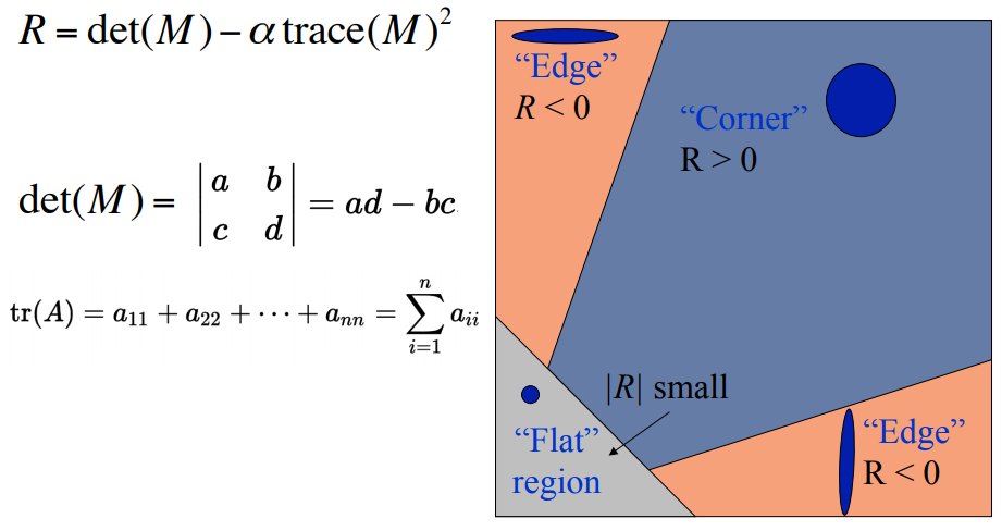
This detection is rotation invariant, but sensitive to changes in scale, viewpoint, and contrast.

We need some way to find the characteristic scale of features. The best mthod to do so is the Laplacian of the Gaussian function, or \(\left\vert{\sigma^2(L_{xx}(x, \sigma) +L_{yy}(x, \sigma ))}\right\vert\)