Computer Graphics

Points, Lines, Vectors, Planes

A linear combination of \(m\) vectors is given by \(\textbf{w} = a_1\textbf{v}_1 + \ldots + a_m\textbf{v}_1\)

An affine combination is a linear combination such that \(\sum_{i=1}^{m}{a_i} = 1\)

A convex combination is a linear combination where \(a_i \geq 0 \text{ for } i=1 \ldots m\)

Homogenous Representation

Vectors and points are represented as \(4 \times 1\) column matrices

\(\textbf{v} = \begin{bmatrix} v_1 \\ v_2 \\ v_3 \\ 0 \end{bmatrix}\) \(P = \begin{bmatrix} P_1 \\ P_2 \\ P_3 \\ 1 \end{bmatrix}\)

The difference of two points is a vector:

\(P = \begin{bmatrix} P_1 \\ P_2 \\ P_3 \\ 1 \end{bmatrix}\) \(Q = \begin{bmatrix} Q_1 \\ Q_2 \\ Q_3 \\ 1 \end{bmatrix}\) \(P - Q = \textbf{v} = \begin{bmatrix} P_1 - Q_1 \\ P_2-Q_2 \\ P_3-Q_3 \\ 0 \end{bmatrix}\)

Lines

There are three main forms for lines:

Explicit representation has trouble representing vertical lines, while implicit representation to check if a point is on (\(f(x,y) = 0\) ), above ( \(f(x,y) > 0\) ), or below (\(f(x,y) < 0\) ) the line.

Parametric makes it easy to draw the line with regards to another paramater, \(t\)

Coordinate Systems

With the homogenous representaiton, we can define coordinate systems. A coordinate system is determined by three linearly independent vectors, \(\textbf{a, b, c}\) and an origin point, \(O\).

We can see the reason behind the 0 and 1 in the homogenous representation to represent vectors and points.

Affine Transformations

The homogenous representation also makes it easy to represent affine transformations as matrix multiplication \(Q = \textbf{M}P\). There are four basic affine transformations, and every other affine transformation is a combination of these four transformations.

Translation

\(\begin{bmatrix} Q_x \\ Q_y \\ Q_z \\ 1 \end{bmatrix} = \begin{bmatrix} 1 & 0 & 0 & T_x \\ 0 & 1 & 0 & T_y \\ 0 & 0 & 1 & T_z \\ 0 & 0 & 0 & 1 \end{bmatrix} \begin{bmatrix} P_x \\ P_y \\ P_z \\ 1 \end{bmatrix}\)

To apply an inverse \(\textbf{M}^{-1} = \begin{bmatrix} 1 & 0 & 0 & -T_x \\ 0 & 1 & 0 & -T_y \\ 0 & 0 & 1 & -T_z \\ 0 & 0 & 0 & 1 \end{bmatrix}\)

Rotation

\(\begin{bmatrix} Q_x \\ Q_y \\ Q_z \\ 1 \end{bmatrix} = \begin{bmatrix} cos \theta & -sin \theta & 0 & 0 \\ sin \theta & cos \theta & 0 & 0 \\ 0 & 0 & 1 & 0 \\ 0 & 0 & 0 & 1 \end{bmatrix} \begin{bmatrix} P_x \\ P_y \\ P_z \\ 1 \end{bmatrix}\)

To apply an inverse \(\textbf{M}^{-1} = \textbf{M}^T\)

This is because, \(\textbf{M}\) is an orthonormal matrix.

Note that with 3D rotation, it is possible to run into gimbal lock, where we lose one degree of freedom.

Scaling

\(\begin{bmatrix} Q_x \\ Q_y \\ Q_z \\ 1 \end{bmatrix} = \begin{bmatrix} s_x & 0 & 0 & 0 \\ 0 & s_y & 0 & 0 \\ 0 & 0 & s_z & 0 \\ 0 & 0 & 0 & 1 \end{bmatrix} \begin{bmatrix} P_x \\ P_y \\ P_z \\ 1 \end{bmatrix}\)

To apply an inverse \(\textbf{M}^{-1} = \begin{bmatrix} \frac{1}{s_x} & 0 & 0 & 0 \\ 0 & \frac{1}{s_y} & 0 & 0 \\ 0 & 0 & \frac{1}{s_z} & 0 \\ 0 & 0 & 0 & 1 \end{bmatrix}\)

Shear

\(\begin{bmatrix} Q_x \\ Q_y \\ Q_z \\ 1 \end{bmatrix} = \begin{bmatrix} 1 & a & 0 & 0 \\ 0 & 1 & 0 & 0 \\ 0 & 0 & 1 & 0 \\ 0 & 0 & 0 & 1 \end{bmatrix} \begin{bmatrix} P_x \\ P_y \\ P_z \\ 1 \end{bmatrix}\)

To apply an inverse \(\textbf{M}^{-1} = \begin{bmatrix} 1 & -a & 0 & 0 \\ 0 & 1 & 0 & 0 \\ 0 & 0 & 1 & 0 \\ 0 & 0 & 0 & 1 \end{bmatrix}\)

Projection Transformations

A projection is basically a mapping from \(R^n \rightarrow R^m\) where \(n > m\)

There are many different types or projections

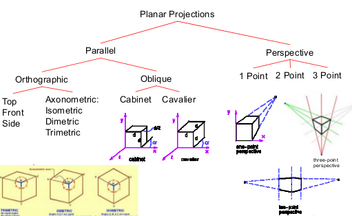
Basic Orthographic Projection

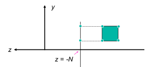
Perspective Projection

View Volumes

Viewports undo the distortion of the projection transformation and map pixel coordinates on screen.

Wireframe Displays

Compute $$M_mod$$
Compute $$M^{-1}_cam$$
Compute $$M_{modelview} = M^{-1}_{cam} M_{mod}$$
Compute $$M_O$$
Compute $$M_P$$
Compute $$M_{proj} = M_OM_P$$
Compute $$M_{vp} = M_OM_P$$
Compute $$M = M_{vp}M_{proj}M_{modelview}$$

for each line segment $$i$$ between $$P_i$$ and $$Q_i$$ do
    $$P = MP, Q=MQ$$
    drawline($$P,Q$$)

Line Rasterization

We want to convert everything into pixels, including lines.

Bresenham Midpoint Algorithm - maps line to pixels using the implicit form of the line and provides a fast way of choosing the next pixel.

void drawLine(int x1, int y1, int x2, int y2)
{
    int x, y, dx, dy, d, dE, dNE;
    dx = x2-x1;
    dy = y2-y1;
    d = 2*dy-dx; //start point
    dE = 2*dy; //if we move one pixel east, the distance from the line is increased by dy
    dNE = 2*(dy-dx) //if we move one pixel northeast, the distance from the line is  increased by dy - dx
    y = y1;
    for (x=x1; x<=x2; x++)
    {
        SetPixel(x,y);
        if (d > 0) // next closest pixel is the NE pixel
            d = d + dNE;
            y = y + 1;
        else //next pixel is the E pixel
            d = d + dE
    }
}

To fill simple polygons, use the recursive Flood-Fill Algorithm.

public void floodFill(int x, int y, int fill, int boundary)
{
    if (x<0 || x>=width)) return;
    if (y<0 || y>=height)) return;

    if (getPixel(x,y) != fill && getPixel(x,y) != boundary)
    {
        setPixel(x,y,fill);
        floodFill(x+1,y,fill,boundary);
        floodFill(x-1,y,fill,boundary);
        floodFill(x,y+1,fill,boundary);
        floodFill(x,y-1,fill,boundary);
    }
}

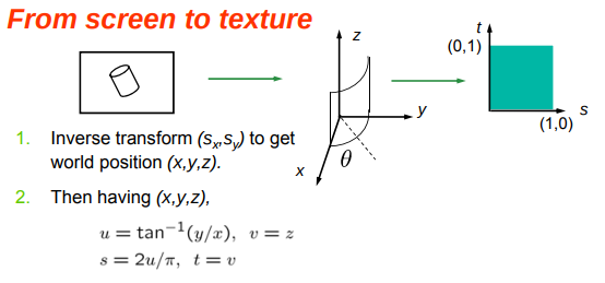
Texture Mapping

\((S_x, S_y) = T_{ws}(T_{tw}(s,t))\)

Textures are always images paramaterized by \((s,t)\)

A better approach is to go from the screen to texture to avoid calculating pixel coverage. \((s,t) = T_{wt}(T_{sw}(S_x,S_y))\)

This approach only works for vertices, so we can calculate texture coordinates by interpolation along interior points.

However, when coupled with a prespective projection, this causes distortion, since the steps are not all equal.

To make it work properly, we must do the perspective division after the interpolation across the polygon.

Visibility

In order to improver performance, we don’t want to draw polygons we can’t see. An object is not visible if

• Outside the view volume
• Self-occlusion
• Object-object occlusion

Clipping and Culling

Clipping is done in the CCS, we clip anything not in the 4D projection volume by finding the intersection between lines and planes and using that to restrict the paramtaterization paramter \(t\).

Culling occurs when an entire polygon is outside of the view volume.

Backface Culling

Any backfacing polygons won’t be seen by the camera. We can efficiently do this by using the z-coordinate of the normal vector if it is an orthographic projection.

Culling in the VCS

• Calculate the normal \(\textbf{n} = [a,b,c]^T\) and the plane equation \(P\)
• if \(P(eye) >0\) that means that the eye is above the plane - front facing
• if \(P(eye) < 0\) that means that the eye is below the plane - back facing

Visibility Algorithms

Image-space Algorithms - operate on pixels/scan-lines e.g. Z-buffer

Object-space Algorithms - BSP, variations on the Painter’s Algorithm. \(O(n^2)\) time

Z-Buffer Algorithm

we generate z values along a scan line from either the plane equation or bilinear interpolation

for all i,j
{
    Depth[i,j] = MAX_DEPTH
    Image[i,j] = BACKGROUND_COLOR
}
for all polygons P 
{
    for all pixels in P 
    {
        if (Z_pixel < Depth[i,j]) 
        {
            Image[i,j] = Color_pixel
            Depth[i,j] = Z_pixel
        }
    }
}

One drawback with Z-buffer is that there is only one visible surface per pixel, which makes it hard to do transparency.

We can use A-buffer instead, which contains assigns the average value of a linked-list of surfaces .

Binary Space Partition Trees

BSPtree *BSPmaketree(polygon_list) {
    choose a polygon as the tree root
    for all other polygons
        if polygon is in front, add to front list
        if polygon is behind, add to behind list
        else split polygon and add one part to each list

BSPtree = BSPcombinetree(
    BSPmaketree(front_list),
    root,
    BSPmaketree(behind_list) )
}

Depth Sorting Algorithms

• sort polygons by z
• resolve ambiguities where z-extents overlap
• scan-convert polygons in back-to-front order

Ambiguities are resolved by exchanging the order of surfaces or by creating new polygons that split up ambiguities.

Scanline Algorithms

for each scanline (row) in image
    for each pixel in scanline
        determine closest object
        calculate pixel color, draw pixel
    end
end 

Less memory intensive and can handle multiple polygons.

Shading

There are blocked, wireframe, and shaded rendering styles.

Light is usually emitted from light sources and reflects off of surfaces. Some light is absorved, some reflected, and some refractable

Light is characterized as RGB triples, and we operate on each channel independently.

There are two types of reflection: Diffuse and Specular reflection.

Diffuse Reflection

Models dull, matte surfaces like chalk.

Calculated via Lambert’s Law. \(I = I_L k_d cos\theta = I_L k_d(\textbf{n} \cdot \textbf{L})\) Where \(I_L\) is the initial light source intensity and \(k_d\) is the diffuse coefficient.

Specular Reflection

Models shiny surfaces, most surfaces are imperfect specular reflectors (a combination of diffuse and specular reflection).

The Phong Model

Purely empirical model. \(I = I_L k_d cos\theta + I_L k_s {cos}^n \phi = I_L k_d(\textbf{n} \cdot \textbf{L}) + I_L k_s (\textbf{r} \cdot \textbf{v})^n\)

Where \(n\) is the “shininess factor”, \(k_s\) is the specular coefficient, and \(\phi\) is the angle between viewing and reflection.

Blinn-Torrance Specular Model

This agress better with experimental results.

\(I_S = I_Lk_s(H \cdot V)^n\) where \(H\) is the halfway vector, or \(\frac{L+V}{\|L+V\|}\)

However, areas that are not directly illuminated appear black, which is not natrual.

We can add a ambient glow term to our equation \(I = I_L k_d cos\theta + I_L k_s {cos}^n \phi + I_ak_a\) where \(I_a\) is the ambient light intensity and \(k_a\), which is a reflectance coefficient.

Types of Shading

Illumination equations are evaluated at surface locations, so we can evaluate at once at each polygon, which is called flat shading.

We can also evaluage it at every vertex and interpolate over the polygon, which is Gouraud Shading.

Phong shading takes this one step further by interpolating normals over each polygon and evaluating the illumination at each pixel.

We can deal with perspective distortion by using byperbolic interpertation. Furthermore, if we don’t have smooth normals, colors may change if the polygon order changes.

This model also fails to account local phenomena, like shadows, attenuation, and transparent objects. Furthermore, global illumination is just approximated but not represented in our code.

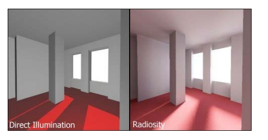
Global Illumination

To approximate global illumination, we can use Radiosity.

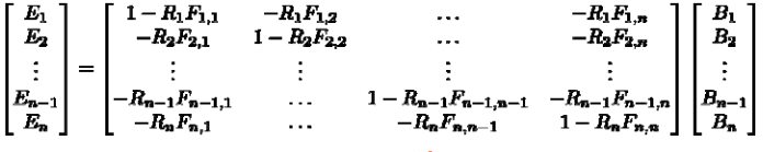
First we break the scene down into small patches, and assume unifrom reflection and emission per patch. Since Light Leaving = Emitted Light + Reflected Light

\(B_iA_i = E_iA_i + R_i \sum_j{B_jF_{j,i}A_j}\) where \(B_i\) is the flux density.

We can then compute form factors \(F_{i,j} for 1 \leq i, j \leq n\) and then solve a system of linear equations.

Ray Tracing

The light that point \(P_A\) emits comes from

• light sources
• reflection from other objects
• refraction from other objects

Diffuse objects only receive light from light sources. Ray tracking works best for specular and transparent objects.

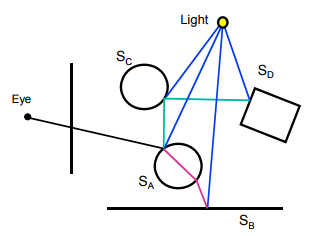
It is easiest to trace rays backwards from eye to scene (eye-based), but it is possible to trace from source to eye (light-based).

  For each pixel on screen:
  	determine ray from eye through pixel
  	find closest intersection of ray with an object
  	cast shadow rays to light sources
  	recursively cast reflected and refracted ray
        calculate pixel color
        paint pixel

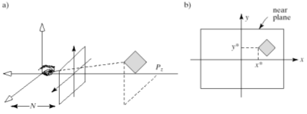
Setting the camera and the image plane

A pixel in the near plane \(P(r,c) = (u_c, v_r)\) where \(u_c = -W + W \frac{2c}{N_c-1}\) and \(v_r = -H + H\frac{2c}{N_r-1}\)

To find the ray through a pixel, use the parametric form of a line. \(ray(r,c,t) = eye + t(P(r,c) - eye)\)

We know that in the world coordinate system: \(P(r, c) = eye - N\textbf{n} + u_c\textbf{u} + v_r\textbf{v}\)

hence \(P(r,c) = eye + t(-N\textbf{n} +u_c\textbf{u}+v_r\textbf{v})\)

Finding Ray-Object Intersections

\(ray(t) = S + t\textbf{c}\)

We can solve this for the two solutions (if two exist) and take the one with the smaller \(t\) value to get the first intersection.

Transformed Primitives

Intersect the inverse-transformed ray with the untransformed primitive.

Shadow Rays

Intersect each shadow ray with all objects, apply illumination if not intersection.

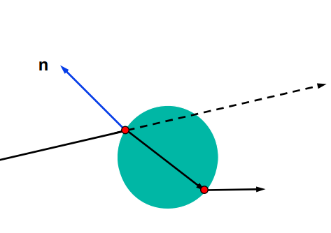
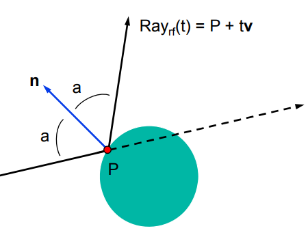
Reflected Rays

\(Ray_{reflected} = P + t\textbf{v}\) where \(\textbf{v} = -2(\textbf{n} \cdot \textbf{c})\textbf{n} + \textbf{c}\)

Refracted Rays

Calculate this using Snell’s Law.

Can be improved upon with participating media, translucency, sub-surface scattering, aperture effects, depth of field, or photon mapping.

Sampling and Reconstruction

Aliasing in Graphics

One way to handle aliasing is to blur the image. Either prefiltering (before sampling) or postfiltering (after sampling)

Prefiltering - use average intensity of square pixel area.

Bresenham’s Algorithm helps improve pixel coverage.

Filtering

Filter the step function using a convolutional kernel \(g\).

We can use a box filter, but the problem is that area coverage is independent of position.

Instead, we can use a Barlett Window.

Supersampling

Take a lot of samples, and then combine them

We can do this stochastically

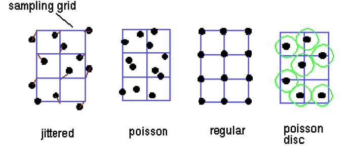
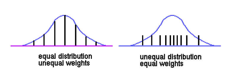
We can also weight each sample to give them relative importance.

Color

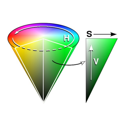
We see color via cones in our eye. There are three types of cones (SML) that correspond to RGB respectively.

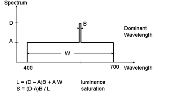
hue is determined by the dominant wavelength.

luminance determined by total power of the light.

saturation is the percentage of luminance in the dominant wavelength.

RGB color model.

Represent colors a vector of three weights, \(w_r, w_b, w_g\) that are all from 0 to 1.

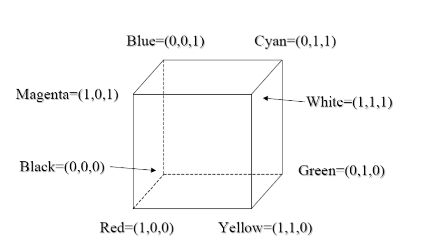
If we intersect this cube with the \(r+g+b=1\) plane, we get the saturated color curve.

Color Matching

Aren’t able to produce all wavelengths of light, so we try to match the distriution as best as possible. However we cannot keep negative coefficients, so we restrict this to an affine combination of (r,g,b)

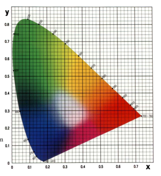
However, we cannot create all of the color scope with RGB. We are limited to the RGB Color gamut.

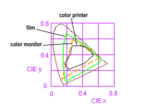
Additive and Subtractive Color

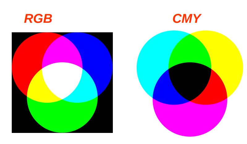
CRTs and other computer displays are an additive model, while printer ink (CMY) is a subtractive model.

Color conversion

We can use the CIE conversion to convert colors between two screens.

Geometric Modeling

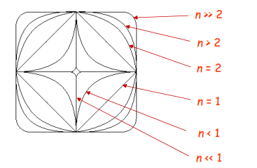
Supercircle

Implicit form: \(\frac{x}{a}^n + \frac {y}[b]^n = 1\) Parametric form: \(x(t) = a cos(t)\left\vert{cos(t)^{frac{2}{n-1}}}\right\vert\) \(y(t) = a sin(t)\left\vert{sin(t)^{frac{2}{n-1}}}\right\vert\)

Drawing Parametric Curves

We can compute some points \(p_i = p(t_i) = (x(t_i), y(t_i))\) and then draw a line between each line to approximate the curve.

We use parametric polynomials and constrain them to create desired curves by splining togethere piecewise parametric curves.

Bezier Curves

Use the De Casteljau Algorithm to generate curves.

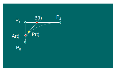
\(A(t) = (1-t)P_0 + tP_1\) \(B(t) = (1-t)P_1 + tP_2\) \(P(t) = (1-t)A(t) + tB(t)\)

These curves are invariant under affine transformations, and also uphold the Convex Hull property and the Variation dimininishing property - which states that no straight line cuts the curve more than it cuts the control polygon.

In 3D, Bezier curves can be written as follows:

Cubic Bernstein Polynomials.

Cubic version of general Bernstein polynomials, which is an expansion of \([(1-t) + t]^L\) where \(L\) is the degree of the polynomial.

These polynomials are always positive and are zero onlyt at \(t=0,1\).

This is an affine combination of points.

Cubic curves give us a good mixture of flexibility and computational simplicity. We can create more complex curves by stiching these curves together piecewise.

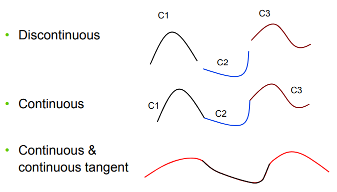
Continuity of Curves

Parametric continuity - \(C^k\) means that each piecewise function is differentiable \(k\) times.

Geometric continutity - \(G^k\) means that the curve itself is differentiable \(k\) times - that means that two segments meet at the same point/have same tangent depending on \(k\).

In 3D, we can write a curve as follows

Hermite Curves

Specify endpoints and tangent vectors and endpoints. Easy to paste together and gaurentees \(G^1\) continuity.

We can convert Bexier curves to Hermite curves by making sure the tangents are the same, that is

Advanced Splines

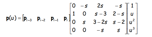
Catmull-Rom Splines interpolate the points and proved \(C^1\) continuity.

Usually used with some tension parameter \(s\).

B-Splines curves no longer interpolate control points. Is \(C^2\) continuous with no invariance under prespective projection.

Nonuniform Raional B-Splines can be used to provide invariance under perspective projection and can create exact conic sections.

Ideally, blending functions

• have sufficient smoothness
• eacy to compute and stable
• should sum to unity over [a,b]
• should have support over a portion of [a,b]
• should be able to interpolate certain control points

Modeling Surfaces

Surfaces are usually modeled parametrically \(\textbf{p}(u,v) = \begin{bmatrix} x(u,v)\\y(u,v)\\z(u,v)\end{bmatrix}\)

We can compute two tangent vectors, \(\textbf{p_u} \textbf{p_v}\) and then take the cross product to get the normal vector.

Height Fields

\(z = f(x,y)\)

Some examples include the Gaussian function and the Sinc function

Ruled Surfaces

Convex combination of two curves. There is some line that entirely on the surface that passes through every point.

Generalized Cone - \(P(u,v) = (1-v)P_0 + vP_1(u)\), where \(P_0(u) = P_0\).

Generalized Cylinder - \(P(u,v) = (1-v)P_0 + v(P_0+d) = P_0(u) + vd\) where \(P_1 = P_0 + d\).

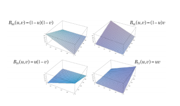
Bilinear Path - \((1-v)(1-u)P_{00} + (1-v)uP_{01} + v(1-u)P_{10} + vuP_{11}\) where \(P_1, P_0\) are both lines.

Surfaces of Revolution

Sweep a profile curve around an axis.

Tensor Product Patches

Generalized form of our spline patches.

Spline Curve - \(\textbf{p}(u) = \sum_{i=0}^{n}{\textbf{p}_iB_i^n(u)}\)

Spline Patch - \(\textbf{p}(u,v) = \sum_{i=0}^{m}\sum_{j=0}^{n}{\textbf{p}_{ij}B_{ij}^{mn}(u, v)}\)

We can write each basis function as a function of two 1-D basis functions, so

Again, we can use the de Casteljau Algorithm to generate Bezier Patches.

These surfaces are affine invariant, and uphold the convex hull, planer percision, and variation diminishining limitations seen before.

We can also stich cubic Bezier surfaces together piecewise to get a more complicated surface.

Similarily, we also have Hermite Surfaces but these now take in the position, tangent and twist of the endpoints.

Modeling Objects with Patches

Ideally, we want to paste together multiple patches to cover an entire object.

To do this, we should transform complicated surfaces into simple primitives - triangles, quadrilaterals, etc.

We can vary the paramter \(u\) from 0 to 1 and connect corresponding points by plugging them into a position function. However, this does not gaurentee uniform spacing in the position space. Furthermore, control over the length is very important to tune.

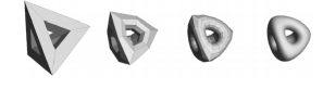
Modeling via Subdivision.

Start with control polynomial
Recursively subdivide until smooth
Draw individual line segments

We need two fundamental operations: linear subdivision - introducing new vertices by splitting each edge at its midpoint.

linear smoothing - modify positions of vertices by smoothing via a weighted average of neighbors. \(v_i = \begin{bmatrix}v_{i-1} & v_i & v_{i+1}\end{bmatrix} \begin{bmatrix} \alpha_1 \\ \alpha_2 \\ \alpha_3 \end{bmatrix}\)

The final shape of the curve is determined by the weights of the matrix.

We can see that this is a linear operation, as each point is a linear combination of the points before. \(P_k = P_{k-1}S_{k-1}\)

To apply this to surfaces, we can split face into four quadrilaterals and then compute the barycenter around each vertex.

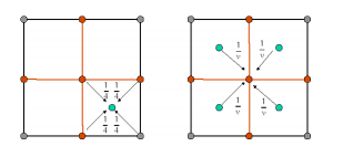
extraordinary points exists when points have more than 4 edges/faces connected to them.

All in all, subdivision lets us represent surfaces well, and are easy to scale to the ideal resolution.