So this summer I officially started doing research with UCLA-NLP.

My research this summer has been mainly focused on sentence embeddings. That is finding a function that maps a sentence (for our purpose a sequence of tokens) $S = [1, 10, 15, \ldots 5, 6 ]$ to a vector $v \in \mathbb{R}^d$.

Sentence embeddings are a key part of many NLP pipelines. Finding good representations is essential for machine learning - without good representations, we can’t fit models properly to our data. For some empirical justification that representations matter, we can look at computer vision. For some applications converting the color space from RGB to LAB increases the accuracy of deep neural networks [¹], even though it’s the exact same data.

My work this summer can be broken down into three main categories:

1. Comparing sentence embedding techniques on real-world data.
2. Trying different fine-tuning approaches.
3. Trying to combine BERT with a contrastive loss.

I just want to make a huge disclaimer here that these results are not rigorous at all and were mainly used to evaluate the feasibility of different approaches, and not as concrete baselines. Also I want to thank Professor Kai-Wei Chang and my research partner Di Qu, who were both very helpful.

Comparing different sentence embeddings on industry data

Taboola graciously provided several news datasets, which I used to compare several different embedding techniques.

The first dataset the provided consisted of the first sentence of news articles, as well as extracted entities in free form text, along with a taxonomy (think news/politics/us/iraq-war). The second dataset also consisted of a short blurb from the article, but this time instead of the taxonomy, we had the section label - which corresponds to the section of the website where the article was found - something like Women's Health. The top-level taxonomy dataset was around 2M lines, while the section dataset contained ~30k lines.

Taboola provided a doc2vec model as a baseline, which was their current production model. I compared the performance of two different models:

• QuickThoughts[²] - a discriminative sentence representation approach. Quickthoughts uses contrastive learning and mines related samples by taking samples close together as semantically similar, while sentence that are far apart are considered semantically dissimiliar. It is trained on the BookCorpus dataset, which is around 68 million lines. Quickthoughts relies on two encoders, which in this case were bidirectional GRU-RNNs. At evaluation time we usually either average, concatenate, or discard one of the encoders. For all my runs the two encodings were averaged together.
• BERT[³] - a deep transformer language model that has set several SOTA benchmarks. BERT is pretrained by masking a certain percentage of tokens, and asking the model to predict the masked tokens. There is also a next sentence prediction task, where a pair of sentences are fed into BERT and BERT is asked to determine whether these two sentences are related or not. This NSP task is very similar to the QT learning objective. To get sentence embeddings, we can take the mean of all the contextualized word vectors or take the CLS token if the model has been fine-tuned.

Both of these models can be fine-tuned by fitting a softmax layer on top, and training the model further with a small learning rate. This allows the model to be adapted to the domain-specific task. We compared the performance of both QT and BERT fine-tuned on 20% of the dataset, which is about 420k lines for the top-level taxonomy and about 10k lines for the section dataset.

Results

To compare embedding performance across these two datasets we trained a softmax classifier on top of the embedding provided, trying to predict both the top level taxonomy (20 categories) and the section label (14 categories). We looked at the training and test accuracy of these classifiers.

We were also curious as to the clustering performance of these representations, so we ran k-means with $n_{clusters} = n_{categories}$ on each dataset. After that, we compared the adjusted rand index and adjusted mutual information scores of the clusters, using the provided top-level taxonomy/section label as the ground truth.

Top-Level Taxonomy

Model	Rand Index	Adjusted MI	Train accuracy	Test accuracy
Taboola D2V	9.85%	17.22%	49.81%	48.13%
QuickThoughts	10.37%	17.73%	56.15%	54.11%
QuickThoughts (fine-tuned on 420k lines)	22.15%	30.12%	62.42%	59.74%
BERT-CLS	8.88%	15.70%	53.20%	51.55%
BERT-mean pooling	8.31%	15.77%	54.87%	54.17%
BERT-CLS (fine-tuned on 420k lines)	26.83%	32.99%	62.21%	53.88%

Section

Model	Rand Index	Adjusted MI	Train accuracy	Test accuracy
Taboola D2V	6.99%	8.12%	53.37%	44.41%
QuickThoughts	5.95%	9.24%	67.84%	52.80%
QuickThoughts (fine-tuned on 10k lines )	12.52%	19.84%	72.00%	57.82%
BERT-CLS	2.25%	6.01%	33.20%	30.88%
BERT-mean pooling	1.82%	5.04%	29.30%	26.08%
BERT-CLS (fine-tuned on 10k lines )	38.56%	42.55%	76.93%	68.92%

Right of the bat we can see that our embedding techniques perform much better than Taboola’s doc2vec model. For some reason, the pre-trained BERT model performed extremely poorly on the Section dataset, although once it was fine-tuned it had the best performance.

We also see a marked improvement when fine-tuning our models, both in our clustering metrics as well as our classification metrics. This is because our classification CE loss should force the points that are labeled the same to be as far away from each other as possible, which helps our clustering perform well.

Comparing different fine-tuning approaches:

Given that fine-tuning had a large impact on our performance, I wanted to see if there were different ways to fine-tune the model.

The standard approach to fine tune BERT is to add a linear layer and softmax on the CLS token, and then training this new model using your standard CE loss[³], backpropagating through all layers of the model.

This approach works well and is very explicit, but there are some problems with it. Firstly, there’s some variability when fine-tuning with a small corpus, and sometimes one will need to restart the fine tuning [³]. In addition, one may run into problems with catastrophic forgetting, as we don’t gradual unfreeze the layers like UMLFit[⁴]. This kind or problem is usually okay though, because if the corpus we’re fine-tuning on is small, it’ll be fast to fine-tune and we can just fine-tune multiple times and take the best run.

I wanted to try several different fine-tuning approaches, although these approaches don’t really address the problems I mentioned above. Moreso I was curious as to weather I could be less explicit with my fine-tuning objective. That is, since the fine-tuning task and the evaluation task are the same, if we get good fine-tuning performance, it makes sense that we get good evaluation performance.

But do there exist other fine-tuning tasks that are not equivalent to the evaluation task but still lead to better evaluation performance? And if so why?

With this in mind, I tried two different fine-tuning approaches:

Hierarchical fine-tuning

The idea here is come from some experiments that my research partner Di ran.

On the 20 newsgroups dataset he noted a increase in training/test accuracy when fine-tuning on the just top level labels. He fit a softmax layer, but restricted it to just the 7 top-level categories instead of the full 20 categories. However, at test time, a full 20 category softmax layer is fit to the model.

The idea here is that the updates made to the underlying BERT model when fine-tuning on just the top-level categories yields a representation that performs better on the 20-category softmax versus the baseline.

But the one thing that peeved me about this is that the label encodings share no information between fine-tuning and evaluation. That is the top level category misc is encoded to 4 when fine-tuning but is encoded to 6 in the second scheme (these numbers are arbitrary, they’re just here to show the problem).

I thought it would be more natural to use a hierarchical encoding scheme. That it we should encode a category computers.graphics as the vector $[1, 1]$ and computers.asdf.mac as $[1, 2]$ instead so that there’s some notion of similarity between the labels.

Unfortunately, this idea wasn’t very fruitful at all, and I saw no difference between fine-tuning with hierarchical softmax and a normal flat softmax.

Contrastive Fine-Tuning of BERT

The central idea behind a contrastive loss is that given two samples, $x^+$, $x^-$, we’d like for $x^+$ to be close to x and for $x^-$ to be far away from x.

The key idea of this approach is how to mine these semantically similar examples. Since we have the labels of the dataset, I did this by encoding the entire batch, and then specify that all samples that occur within in the same class are semantically similar, while all the examples that are from different classes are distinct.

Of course, we also need to then calculate a targets matrix to compute a KL divergence and get a loss between these two matrices.

Ideally our targets matrix $T \in \mathbb{R}^{n \times n}$, where $n$ is the batch size , would be such that \(T_{i, j } = 1\) if $y_i == y_j$ and $0$ otherwise. Then we can take a row-wise softmax and KL divergence between the targets and encoding matrix to get our loss. (See the Implementation Details section here for a more thorough explanation.)

There’s a pretty clever way to do this - Note that if we one hot encode our label, $y \in {0 \ldots n_{cat}}$, into $Y$, a one hot vector, we can see if two samples are in the same class by dotting the two one hot vectors together.

If the two vectors are the same, the dot product will be 1, however, if these labels are different then the one hot labels dotted together will be 0.

So to do this batch-wise, we can one-hot encode our labels vector into a one hot matrix, and then take the dot product of this matrix and it’s transpose in order to get our targets matrix. This can be done very easily using the OneHotEncoder function in scikit-learn[⁵].

Results

I ran all my experiments using the 20newsgroups dataset. I compared the training and test accuracy of four different models. For both fine-tuned models, I used a learning rate of 5e-5 and a batch size of 32 on 20% of the dataset. To give a fair comparison between the normal fine-tuning and the contrastive model, I discarded the softmax layer used to fine-tune normally and trained a new softmax layer on top in order to get the training/test accuracy. All fine tuning and BERT experiments were done on the CLS token.

1. QuickThoughts - This is the normal quickthoughts model
2. Normal BERT model
3. Normal BERT model + normal BERT fine-tuning
4. Normal BERT model + contrastive fine-tuning

Model	training accuracy	test accuracy
QuickThoughts	55.50	54.72
BERT	58.56	45.36
BERT + normal fine-tuning	82.61	68.48
BERT + contrastive fine-tuning	74.12	53.29

So this contrastive fine-tuning had a positive effect on performance, particularly training accuracy, although it was not as effective as the normal explicit approach.

Although I’m not 100% sure, I have a couple of ideas that might explain this performance gap:

1. First off, there’s an optimization wrinkle here. Since both encodings come from the same encoder, when we backpropagate, the gradients for the model can be quite large, and we need to clip them. Usually contrastive learning uses two encoders for this reason (see word2vec[⁶], quickthoughts[²]), and we either average, concatenate, or discard one of the encodings.

2. Another problem with the contrastive loss is that it can be a bit too greedy, as it will try to force all of the related example to occupy the same place in the embedding space. But obviously, even semantically similar examples differ from each other a bit. This is the idea behind triplet losses, which just seek to operate on a single anchor, positive, negative example triplet. [⁷]

Ultimately, while this contrastive loss was helpful (it led to higher train and test accuracy), one could get better performance by taking the conventional fine tuning approach. But given that fine-tuning in this contrastive method did improve performance, I was curious as to what would happen if I incorporated this into the BERT training objective.

ContraBERT

That is, take BERT embeddings as the input into a model trained using contrastive loss. This is very similar as before, but instead of using this contrastive loss for fine-tuning, we’re training BERT for a long period of time in order to get good sentence representations.

Unfortunately I don’t have the computational resources to train BERT from scratch, so instead I tried to a period of very long fine-tuning. That is I initialized BERT from the base model, and then “fine-tuned” over BookCorpus, which was 68 million lines. However, unlike the previous fine-tuning approaches, the fine-tuning data is not representative of the evaluation domain.

That is before we were fine-tuning with data from our evaluation domain, but now our fine-tuning data is just general. I thought this would be a good proxy for evaluating the performance of BERT trained with these objectives.

There were three different approaches I attempted:

1. fixed BERT-QT - this is a feature extraction approach, by just taking the output of BERT and feeding it into a GRU-RNN in order to get out two different embeddings. I then trained the model by minimizing the KL between each row-wise softmax and the targets matrix from QT that represents the next sentence.
2. fluid BERT-QT - this model is the same as above, but instead of fixing the BERT layers, we backpropagate through them. We still feed the output of the BERT model into two GRU-RNNs.
3. ContraBERT - Here we get rid of the GRU-RNNs and instead take our two encodings by taking the CLS token embedding as well as the SEP token embedding (the first and last token respectively). We then do a contrastive loss with these two encodings, and backpropagate through all of BERT.

Results

To compare these different methods I ran several semantic textual similarity benchmarks. These benchmarks encode the dataset into the embedding space and then use cosine distance to try and determine semantic similarity You’ll note that average/CLS BERT embeddings on STS tasks seems to perform poorly. In fact they perform worse than average GloVe word vectors. I took the baseline metrics from Sentence BERT[⁸].

	STS12	STS13	STS14	STS15	STS16
BERT CLS (from [8])	0.201	0.300	0.201	0.368	0.388
QuickThoughts	0.369	0.347	0.352	0.384	0.382
fixed BERT-QT	0.402	0.311	0.345	0.274	0.417
fluid BERT-QT	0.496	0.301	0.437	0.524	0.508
ContraBERT	0.521	0.651	0.608	0.644	0.639
Sentence BERT(from [8])	0.745	0.770	0.731	0.818	0.768

Here’s a training curve for fluid Bert-QT:

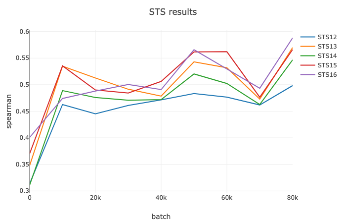
All of the combinations of contrastive learning and BERT do seem to outperform both QT and BERT seprately, with ContraBERT performing the best. So while we’re able to make significant progress compared to BERT and QT baseline models, it’s still not SOTA or comparable to the results found here.

I do want to point out that unlike SentenceBERT[⁸] this is an entirely unsupervised approach - whereas their method relies on the MNLI dataset, which provides labeled pairs of sentences.

There’s a couple of ways I think one could improve performance here:

• I think that we can do some masking on the targets matrix: Basically we hold that every sentence not in the context is a negative sample, but this is a bit of a strong assumption. It might be a bit better to mask out the sentences in a larger context (say 15) window, and only take sentences outside as semantically dissimilar, which may lead to a cleaner negative sample. The CURL framework paper by Arora et al. [⁹] shows how having mislabeled examples may negatively affect performance.
• Hyperparameter tuning. I first tried to train ContaBERT using the LR form the Quickthoughts paper, and I observed very poor performance. It would be good to do a hyperparameter sweep, but I don’t have the computational resources to do that.

Conclusion

This is kind of just a braindump of ideas. There were just a couple of interesting tidbits I wanted to write down (Computing the same-category targets matrix for example).

I think most of these ideas aren’t necessarily bad, but not very interesting - they’re just the simple extension of existing work, taking pieces here and there. However, I do think it was extremely helpful to essentially try a bunch of random stuff and hope it works. I think I have a new appreciation for just how hard research is.

Right now I’m working on a research idea involving cooccurrence matrices and contrastive learning that has it’s roots in the work I’ve done here. It’s looking a lot more promising/interesting than the stuff above, so fingers crossed.

If you have any questions, comments, or corrections please reach out.

References