Simulated Annealing

This is a post about Simulated Annealing.

The Problem

Simulated Annealing is an optimization technique. It is a probabilistic technique to approximate the global max/min of a function. In this post, I describe how to use Simulated Annealing to solve the Traveling Salesman problem.

The idea of the Traveling Salesman problem is that you have \(N\) cities and you want to find the path of least distance that allows you to visit all the cities and end up at your starting city. (You basically just want to find a cycle) You can read more about this problem if you’re unfamiliar with it here.

Approach

Simulated Annealing works as follows:

1. Start off with some random solution. This is just some random permutation of all the cities

2. Create a neighboring solution. In our case, we choose two vertices and reverse the path along these 2 vertices.

3. If the neighboring solution is better than the current solution, switch. However, if the neighboring solution is worse than the current solution, you still have a chance to switch, given by the equation:

In this case \(e\) is the distance of your current path, \(e'\) is the distance of your neighbor path, and \(T\) is the temperature.

1. Now we decay the temperature by a certain rate.

We simply repeat this until the temperature is less than 1 and then we terminate. The end result we have is our “optimal” solution.

Code

You can see the full code on my github here.

First off, we start by initializing the enviorment, setting the initial temperature, cooling rate, and also the starting path.

    #set up enviorment and create points
    temp, coolingRate = 1000, 0.0002
    locs = np.random.randint(0, 20, size=(num_points,2))

    #create the starting path
    startingPath = np.insert(np.random.permutation(num_points-1) +1, 0, 0)
    currentPath = startingPath
    # array to keep track of the distances
    distance = []

Next, I wrote a function that computes the distance of a path

def computePath(locs, path):
 dist = 0 
    for j in path:
        i = path[j]
        k = path[(j+1) % len(path)]
        point = locs[i]
        point2= locs[k]
        dist += (point[0]-point2[0])**2 + ( point[1]-point2[1])**2
    return dist

I also wrote a function to compute the neighbors of a path

def getNeighbors(path_in):
    path = list(path_in)
    index1, index2 = np.random.choice(path, size=(2,1), replace=True)
    path[index1:index2] = reversed(path[index1:index2])
    return path

Now I can just run this simulation until it terminates ($Temp < 1$)

    while(temp>1):
        neighbor = getNeighbors(currentPath)
        e_prime = computePath(locs, neighbor)
        e_current = computePath(locs, currentPath)

        probability = np.exp((e_current - e_prime) / temp)

        if e_prime < e_current:
            currentPath = neighbor
        elif probability > np.random.rand():
            currentPath = neighbor

        temp *= 1-coolingRate;

Result

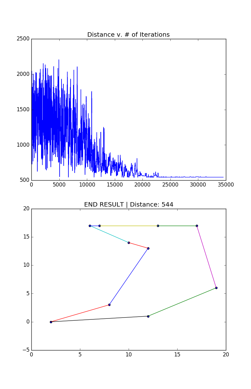
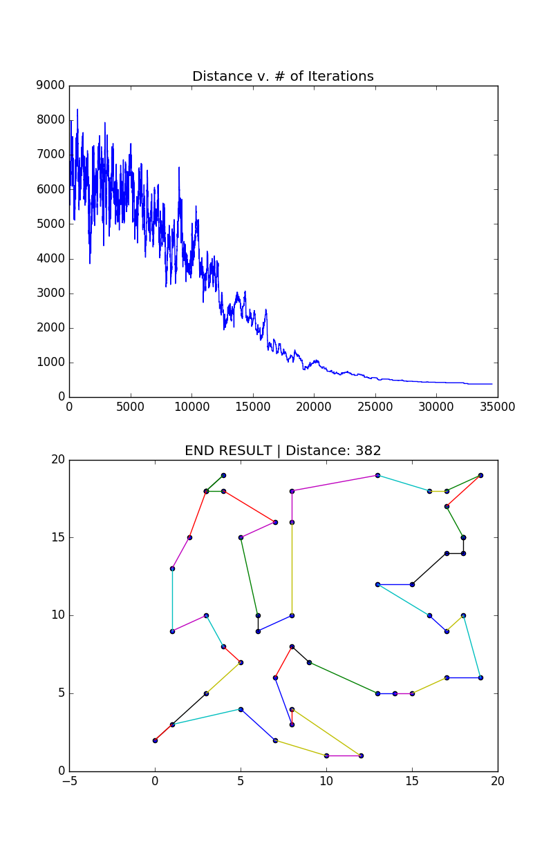
I ended up writing a python program that finds the shortest path along a random set of vertices. I’ve attached the results below.

Example with 10 points

Example with 50 points

This was a quick and fun little project. Later on I’d like to experiment and see if one could use simulated annealing instead of gradient descent to optimize machine learning problems. I think it would be especially effective in cases where you are unable to train for long periods of time. I think it could also be helpful when the search space is especially large - when your model is very complex.