Randomness

Randomness in Algorithms

When you have many good choices, just pick one at random. Randomness can be used to speed up algorithms and ensure good expected runtime.

Linearity of Expectations

Let \(x\) and \(y\) be two random variables. Linearity of Expectations states that

\[E[x+y] = E[x] + E[y]\]

That is, the expected value of the sum is the sum of the expectations.

Quicksort

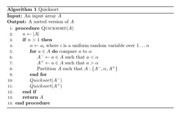
Analysis

Let \(E[T(A)]\) be the number of comparisons. We want to bound \(E[T(A)]\), or the expected number of comparisons that Quicksort will call. We also define \(W(n)\) to be the max expected value of any \(A\) such that the size of \(A\) is \(n\).

From the recurrence relation we see that \(T(A) = T(A^+) + T(A^-) + n-1\)

Taking the expected value of each side yields

\[E[T(A)] = E[T(A^+) + T(A^-) + n-1]\]

We can use linearity of expectations here to break this equation down to

\[E[T(A)] = E[T(A^+)] + E[T(A^-)] + n-1\]

Assume that all elements are distinct, then \(Pr[\left\vert{A^-}\right\vert = i] = \frac{1}{n}\) This is because the pivot must be the \(i+1^{th}\) element, which has probability \(\frac{1}{n}\)

Now we can express the expected value of \(A^-\) as

\[E[T(A^-)] = \sum_{i=0}^{n-1}{Pr[\left\vert{A^-}\right\vert = i] \times W(i)} = \sum_{i=0}^{n-1}{\frac{W(i)}{n}}\]

Similarly, \(Pr[\left\vert{A^+}\right\vert = i] = \frac{1}{n}\)

\[E[T(A^+)] = \sum_{i=0}^{n-1}{Pr[\left\vert{A^+}\right\vert = i] \times W(i)} = \sum_{i=0}^{n-1}{\frac{W(i)}{n}}\]

We can plug this into our previous equation to get

\[E[T(A)] = \sum_{i=0}^{n-1}{\frac{W(i)}{n}} + \sum_{i=0}^{n-1}{\frac{W(i)}{n}} + n-1\]

Remember that \(W(n) = \max{E[T(A)]}\)

\[W(n) \leq \sum_{i=0}^{n-1}{\frac{W(i)}{n}} + \sum_{i=0}^{n-1}{\frac{W(i)}{n}} + n-1 \leq \sum_{i=0}^{n-1}{W(i)} \times \frac{2}{n} + n-1\]

Now we will prove that \(W(n) \leq 2n \log(n)\) by induction

Base Case: \(W(2) = 1 \leq 2 \log(2)\)

Inductive Step: \(W(n) \leq \sum_{i=0}^{n-1}{W(i)} \times \frac{2}{n} + n-1\)

Plugging in the induction hypothesis yields

\[W(n) \leq \sum_{i=0}^{n-1}{2i\log(i)} \times \frac{2}{n} + n-1\] \[W(n) \leq \sum_{i=0}^{n-1}{i\log(i)} \times \frac{4}{n} + n-1\]

Note that \(\sum_{i=0}^{n-1}{i\log(i)} \leq \int_1^n{i \log(i)}\)

Thus \(\sum_{i=0}^{n-1}{i\log(i)} \leq \frac{n^2 log(n)}{2} + \frac{n^2}{4}\)

\[W(n) \leq (\frac{n^2 log(x)}{2} + \frac{n^2}{4}) \times \frac{4}{n} + n-1\] \[W(n) \leq 2n \log(n)\]

Quickselect

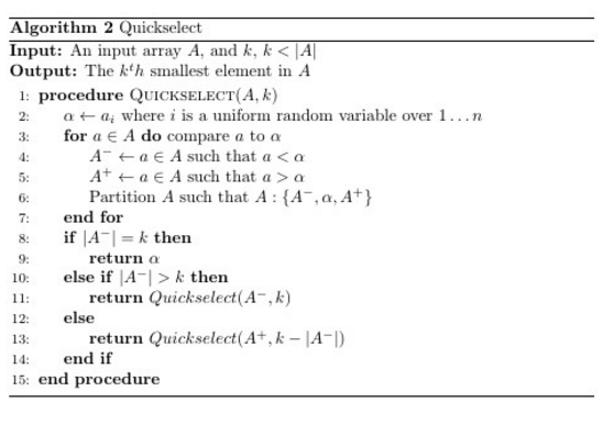
Analysis

Let \(T(A, k)\) be the total number of comparisons that the algorithm makes. We want to bound \(E[T(A,k)]\), which is the expected number of comparisons.

Let \(W(n)\) be the max possible \(E[T(A,k)] \forall A, k \). Let \(B\) be the subarray that Quickselect recursively calls.

We see from the recurrence that \(E[T(A,k)] \leq n + E[W(\left\vert{B}\right\vert)]\)

\[\left\vert{B}\right\vert = \begin{cases} i-1 \text{ if } i > k \\ n-i \text{ if } i < k \\ \end{cases}\]

Dictionaries and Hashing

A Dictionary is a data structure that supports three main operations. For any dictionary \(D\), they will support three basic operations

• INSERT(X) - Insert \(X\) in \(D\) if not present
• DELETE(X) - Delete \(X\) from \(D\) if present
• FIND(X) - Is \(X\) in \(D\)?

We can compare several different data structures and see the advantages of each.

	INSERT	LOOKUP	SPACE
Linked List	\(O(1)\)	\(O(n)\)	\(O(n)\)
Array	\(O(n)\)	\(O(1)\)	\(O(n)\)
Binary Tree	\(O(log(n))\)	\(O(log(n))\)	\(O(n)\)
Dictionary	\(O(1)\)	\(O(1)\)	\(O(n)\)

One way to achieve the time constrainsts of a dictionary is to use Seperate Chaining

In this case, we have an array of size \(n\) and each array has a linked list. We use a random hash function \(h(x): \rightarrow \{1 \ldots n \}\) to assign each element to a linked list, or bucket

Analysis

Let \(Bucket(x) = A[h(x)]\). That is \(Bucket(x)\) returns the bucket where the element \(x\) resides. From this, we can see that the time taken for Inserts/Finds is \(O(\left\vert{Bucket(x)}\right\vert)\). We will try to prove that

\(E[\left\vert{Bucket(x)}\right\vert] \leq 1\) if \(n \geq n^{insert}\)

That is, if the number of inserts we make into the hash table is less than the number of buckets, our hash table will operate with our desired time bounds. Let \(S\) be all the elements inserted into the dictionary \(D\). The size of \(S\) is \(n^{insert}\)

We will create a random variable \(\forall s \in S\)

\[R_s = \begin{cases} 1 \text{ if there is a collision} \\ 0 \text{ otherwise } \end{cases}\] \[E[\left\vert{Bucket(x)}\right\vert] = \sum_{s \in S}{R_s}\]

Using linearity of expectations we get

\[E[\left\vert{Bucket(x)}\right\vert] = E[\sum_{s \in S}{R_s}] = \sum_{s \in S}{E[R_s]}\]

Since our hash function is independently random, the probability of a collision is \(\frac{1}{n}\)

\[E[\left\vert{Bucket(x)}\right\vert] = \sum_{s \in S}{1 \times \frac{1}{n}}\] \[E[\left\vert{Bucket(x)}\right\vert] = \frac{n^{insert}}{n}\]

As we know, \(n^{insert} \leq {n}\), so

\[E[\left\vert{Bucket(x)}\right\vert] \leq 1\]