Learning Better Sentence Representations
19 May 2019 | machine-learning nlpOver the past couple years, unsupervised representation learning has had huge success in NLP. In particular word embeddings such as word2vec and GloVe have proven to be able to capture both semantic and syntactic information about words better than previous approaches, and have enabled us to train large neural end-to-end networks that achieve the best performance on a myriad of NLP tasks.
This post is about contrastive unsupervised representation learning for sentences.
Why learn embeddings?
In unsupervised representation learning, we try to find a function that encodes an example in our dataset, $x \in \mathbb{R}^{n}$ to a lower dimensional vector in $\mathbb{R}^d$. Ideally this smaller vectors captures all of the information we need for some arbitrary downstream task.
But why should we care about learning “good” representations?
One very direct and easy use for these embeddings is semantic search by finding the nearest neighbors of a document in embedding space.
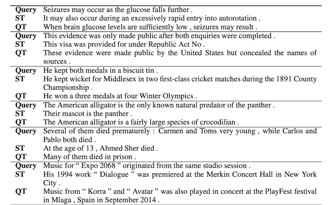
Here you can see nearest neighbor search over a corpus of 1M Wikipedia sentences of both QuickThoughts [1] and SkipThoughts[2], two different embedding approaches.
This type of semantic search is being used more often in industry - recently Microsoft released SPTAG, a library for fast approximate nearest neighbor search. Good embeddings are essential to the performance of these approaches.
Furthermore we can use embeddings to categorize/cluster our data.
Given a small set of representative samples, we can train a simple linear/logistic classifier atop of our embeddings and observe competitive performance on a multitude of binary classification tasks.
For example, at Blend I needed to be able to identify “frozen” comments, comments that directly mentioned app stability issues, in order to improve our application quality. With good sentence embeddings, I was able take a set of $n$ “frozen” comments, and a set of random comments, and create a simple mean classifier that performed better than our existing keyword solution.
Furthermore, we can generalize our approach to learn embeddings to different fields. For example, Asgari and Mofrad [3] trained embeddings for biological sequences (RNA, proteins, etc.). One could also train embeddings for images to implement something similar to Google’s reverse image search.
How can we learn these embeddings?
One common way to learn representations is to train an autoencoder, as done in Skip-Thoughts[2], which used an autoencoder with LSTM-RNN encoders and decoders. The idea is to then throw away the decoder and use just the encoder for embeddings.
Quickthoughts[1], by Leensworn and Lee, seeks to simplify the training process by replacing the generative decoder with a discriminative model.
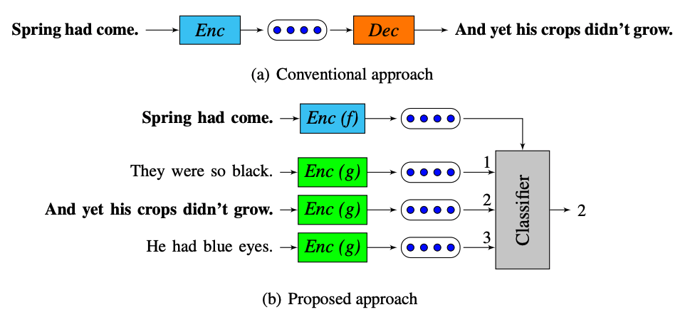
QuickThoughts
Instead of trying to reconstruct our original sentence from our embedding (a), we see to identify a “related” embedding $s_{cand}$ given a set of candidate sentences $S_{cand}$, and a sentence $s$ (b).
This is the central idea of contrastive learning - we seek to be able to identify a similar and dissimilar example given a example. The second half of this post deals extensively with contrastive learning.
The probability that a candidate sentence $s_{cand}$ is related to $s$ is given by
\[P(s_{cand} \mid s, S_{cand}) = \frac{e^{f(s)^T g(s_{cand})}}{\sum_{s' \in S_{cand}} e^{ f(s)^Tg(s') }}\]Here $f$ and $g$ are deep neural networks. The paper explores a wide variety of encoders, but for the sake of simplicity we’ll use GRU networks, taking the last hidden state as the embedding.
This begs the question though - how can we get a large number of pairs of related sentences without labeled data? We do this by exploiting the fact that subsequent sentences in a corpus are likely to be related, and as such we seek to identify the embedding of the next sentence given a candidate set of embeddings.
However, instead of identifying just the next sentence, we seek to identify all the sentences in a context window, which is set as a hyperparameter.
Our training corpus consists of the BookCorpus [4] dataset, a collection of free books. In total it is roughly 68 million sentences long.
Our training objective is then to maximize the probability of identifying each context sentence for each sentence in the training data
\[\prod_{s \in D} \prod_{s_{ctx} \in S_{ctx}} P_\theta(s_{ctx} \mid s, S_{cand})\]If you’re familiar with word2vec then this learning objective may look very similar.
Some implementation details
So now that we have our loss function, let’s figure out how to implement it efficiently.
We’ll use a minibatch of our data as set of candidate sentences, and for the sake of simplicity, we’ll assume that we’re just trying to predict the next sentence. Our modified training objective becomes
\[\prod_{s_i \in D} P_\theta(s_{i+1} \mid s_i, D)\]Let $D$ be one minibatch of sentences, where each sentence $s_i$ is represented by a sequence of word indices, zero-padded to the max sequence length of the minibatch.
\[D = \begin{bmatrix} s_0 \\ \vdots \\ s_n \\ \end{bmatrix} \in \mathbb{R}^{n \times max\_seq\_len}\]First we’ll encode all of the sentences in our minibatch with both encoder networks, as every sentence will be both a context and candidate. Here $h$ is the hidden size of our GRU encoder.
\[enc_f = \begin{bmatrix} f(s_1) \\ \vdots \\ f(s_n) \\ \end{bmatrix} \in \mathbb{R}^{n \times h}, enc_g = \begin{bmatrix} g(s_1) \\ \vdots \\ g(s_n) \\ \end{bmatrix} \in \mathbb{R}^{n \times h}\]Next we can outer product $enc_f$ with $eng_g$ to get our scores matrix - with a small exception. The set of candidate sentences is not suppose to contain $s$, the related sentence, so we need to zero out the scores along the diagonals.
\[scores = \begin{bmatrix} f(s_1) \\ \vdots \\ f(s_n) \\ \end{bmatrix} \begin{bmatrix} g(s_1) \dots g(s_n) \\ \end{bmatrix} = \begin{bmatrix} f(s_1)^Tg_(s_1) & \ldots & f(s_1)^Tg(s_n)\\ \vdots & \ddots & \\ f(s_n)^Tg_(s_1) & & f(s_n)^Tg(s_n) \\ \end{bmatrix} \in \mathbb{R}^{n \times n}\] \[scores_{zero} = \begin{bmatrix} 0 & f(s_1)^Tg(s_2) & \dots & f(s_1)^Tg(s_n) \\ f(s_2)^Tg(s_1) & 0\\ \vdots & &\ddots \\ f(s_n)^Tg_(s_1) & & & 0\\ \end{bmatrix} \in \mathbb{R}^{n \times n}\]Now if we softmax over each row we can convert our scores to a normalized probability distribution, where $prob_{ij} = \frac{e^{f(s_i)^T g(s_j)}}{\sum_{k=0}^n e^{ f(s_i)^Tg(s_k) }} = P(s_j \mid s_i, D) $ = the probability that $s_j$ is the $s_{i+1}$ given the minibatch of sentences $D$ and context sentence $s_i$
\[prob = \begin{bmatrix} \frac{1}{Z_{s_1}} & \frac{e^{f(s_1)^Tg(s_2)}}{Z_{s_1}} & \dots & \frac{e^{f(s_1)^Tg(s_n)}}{Z_{s_1}} \\ \frac{e^{f(s_1)^Tg(s_2)}}{Z_{s_2}} & \frac{1}{Z_{s_2}}\\ \vdots & & \ddots & \\ \frac{e^{f(s_1)^Tg(s_n)}}{Z_{s_n}} & & & \frac{1}{Z_{s_n}}\\ \end{bmatrix} \in \mathbb{R}^{n \times n}\]Now if our model was perfect, this distribution should look like
\[target = \begin{bmatrix} 0 & 1 & \dots & 0 \\ 0 & \ddots & \ddots & 0 \\ \vdots & & & 1 \\ 0 & & & 0 \\ \end{bmatrix} \in \mathbb{R}^{n \times n}\]To compute our loss we can take a KL divergence between our $targets$ and $prob$ matrices, by treating every row as a probability distribution.
Since there’s only one non-zero probability in the $targets$ matrix, the KL term simplifies nicely. Below we compute a KL between row $i$ of our two matrices.
\[D_{KL}(targets_i \mid\mid probs_i) = \sum_{j=0}^n targets_{ij} \log \frac{targets_{ij}}{probs_{ij}} = 1 (\log 1 - \log probs_{i, i+1}) + 0 ( \ldots) = - \log probs_{i, i+1} = - \log P(s_{i+1 }\mid s_i, D)\]Summing over all of the rows yields $- \sum_{s \in D} \log P(s_{i+1} \mid s_i, D)$, which is the simplified training objective presented at the start of this section, but negated as we minimize our loss function.
Code and Results
This can be done quite easily with a couple lines of PyTorch.
# get the encodings
enc_f, enc_g = qt(data)

# calculate scores and zero out when not in candidate set
scores = torch.matmul(enc_f, enc_g.t())
mask = torch.eye(len(scores)).cuda().byte()
scores.masked_fill_(mask, 0)

# compute log_scores
log_scores = F.log_softmax(scores, dim=1)
# returns ideal target distribution
targets = qt.generate_targets(CONFIG['batch_size'])

#Note even though this is called as  kl_loss(log_scores, targets), it actually computes D_KL(targets, scores)
loss = kl_loss(log_scores, targets)
loss.backward()
optimizer.step()
The full code I wrote for training QuickThoughts from scratch can be found here.
I primarily trained on a NVIDIA V100 GPU on GCP. Training took approximately 6 hours for a single GRU encoder with a hidden size of 1000. I used a context size of 3, batch size of 400, and learning rate of 0.0005. Pretrained GloVe word vectors were used for word embeddings.
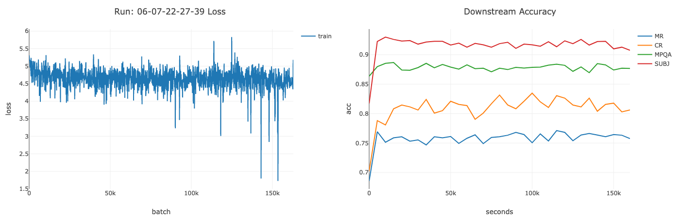
Above you can see the training loss and accuracy of a mix of binary classification tasks over time. I was able to successfully reproduce the results from the original paper, achieving comparable performance on downstream classification tasks.
Why do these embeddings perform so well?
While our approach intuitively makes sense, and empirically performs well, it’s not completely clear how learning to identify the next sentence leads to an embedding that performs well on some classification task.
More generally why does learning to identify related points by minimizing some unsupervised loss lead to a representation that does well on classification tasks down the line?
Arora et al. [5] recently released a theoretical framework for contrastive unsupervised representation learning and were able to show that the unsupervised loss is an upper bound for the supervised loss.
Framework for Contrastive Unsupervised Representation Learning
We assume that we have a distribution $\rho$ over a set of classes $C$, each with a data generating distribution $D_c$.

Then we can think of semantically similar samples as two samples $x, x^+$ from $D_{c+}$, and a semantically dissimilar example $x^-$ from $D_{c-}. This means we can break out our unsupervised loss as follows:
\[L_{un}(f)=\mathop{\mathbb{E}}\limits_{c^+,c^-\sim\rho}\ \mathop{\mathbb{E}}\limits_{x,x^+\sim D_{c^+}}\ \mathop{\mathbb{E}}\limits_{x^-\sim D_{c^-}}\left[\log\left(1+e^{f(x)^Tf(x^-)-f(x)^Tf(x^+)}\right)\right]\]Our supervised loss function between two classes $c_1, c_2$ is the ordinary logistic regression loss between the datapoints generated from each class distribution. The average loss over an arbritary choice of classes is our supervised loss and a measure of the quality of our representation
\[L_{sup}(f)=\mathop{\mathbb{E}}\limits_{c_1,c_2\sim\rho}\ \left[L_{sup}(f, (c_1,c_2))|c_1\neq c_2\right]\]So what is the relationship between $L_{sup}$ and $L_{un}$? Arora er al. were able to show the following:
Lemma: The average classification loss on downstream binary tasks is upper bounded by the unsupervised loss. $L_{sup}(f) \leq \alpha L_{un}(f), \forall f \in \mathbb{F}$
The full proof of this can be found in the paper[5], but it relies on Jensen’ inequality and the convexity of $l$.
Loosely speaking, what this frameworks says is if we manage to find a good representation that minimizes the unsupervised loss, the softmax mean classifier will perform well on some arbritatry downstream classification task, with just a few examples necessary to achieve good performance.
Improving our theoretical bound
One possible improvement that the CURL authors give is to use “blocks” of points, rather than a single positive/negative example.
More concretely, if we seek to minimize
\[L_{un}^{block} (f) := \mathbb{E} \left[ l\left(f(x)^T\left( \frac{\sum_i f(x_i^+)}{b} - \frac{\sum_i f(x_i^-)}{b}\right) \right) \right]\]instead of our conventional unsupervised loss:
\[L_{un} (f) := \mathbb{E} \left[ l \left( f(x)^T \left( f(x^+) - f(x^-)\right) \right) \right]\]we should get better performance on downsteam classification tasks, since this tightens the Jensen’s inequality bound.
This can be done rather simply by applying two convolutions to $enc_g$, one to compute the mean positive sample, $\mu^+$ and one to compute the mean negative sample $\mu^-$.
Interestingly, the Topelitz matrix to compute the convolution for $\mu^+$ is exactly the targets matrix.
Block size = context size?
This got me thinking about the effect that altering our targets matrix (by changing the context_size) and taking a KL divergence would have with regards to this framework. Is this equivalent to the block size modification presented in CURL?
It’d be great if it was the case, as then we could easily implement $L_{un}^{block}$ by just changing the $targets$ matrix, which directly corresponds to changing the context size parameter in QuickThoughts.
We’d like to show that for $b$ similar points $x_1^+, \ldots, x_b^+$ and $b$ dissimilar points $x_1^-, \ldots, x_b^-$ and mean points $\mu^+$ and $\mu^-$.
\[l^{block}_{un}(x, \mu^+, \mu^-) := l^{altered\_targets}_{un}(x, x_1^+ \ldots x_b^+, x_1^- \ldots x_b^-)\]Recall from the above section that we can compute this loss as a KL term.
\[l^{block}_{un} = D_{KL} \left([1, 0] \mid \mid softmax \left( \left[f(x)^T \mu^+ , f(x)^T \mu^- \right] \right) \right)\] \[= \sum_{x \in X} P(x) \left[ \log P(x) - \log Q(x) \right] = - \left( \log e^{f(x)^T\mu^+} - \log \sum_{y \in \{ \mu^+, \mu^ -\}} e^{f(x)^Tg(y)} \right)\] \[= -f(x)^T\mu^+ + \log (e^{f(x)^T\mu^+} + e^{f(x)^T \mu^-} )\]Unfortuanetly this is not the case, as $l_{un}^{altered_targets}$ comes out to a slightly different result.
\[L^{altered\_targets}_{un} = D_{KL} \left([\frac{1}{b} \ldots \frac{1}{b}, 0 \ldots 0] \mid \mid softmax \left( \left[ x_1^+ \ldots x_b^+, x_1^- \ldots x_b^- \right] \right) \right)\] \[= \sum_{x \in X} P(x) \left[ \log P(x) - \log Q(x) \right] = - \sum_{i=0}^b \frac{1}{b}\left(f(x)^Tg(x_i^+) - \log \sum_{j =0}^n e^{f(x)^T g(x_j)} \right)\] \[= -f(x)^T \frac{\sum_ig(x_i^+)}{b} + \log \sum_{j =0}^n e^{f(x)^T g(x_j)}\]These look very similar, but they have a different normalization constant.
Conceptually the block method computes the probability of the mean positive sample given the the mean positive and mean negative sample, while the altered targets approach computes the probability of the mean positive sample given the set of candidate sentences.
Irregardless I was curious wether altering the context size would have an impact on downstream performance.
Comparing Empirical Results
To test this, I trained 4 QuickThoughts models, with a context size of 1, 2, 3, and 4 respectively. The accuracy on several different downstream classification tasks are shown below.
| MR | SUBJ | CR | MPQA | |
|---|---|---|---|---|
| k=1 | 76.71 | 91.74 | 83.95 | 88.61 |
| k=2 | 77.11 | 91.72 | 83.84 | 88.50 |
| k=3 | 76.54 | 92.18 | 83.34 | 88.45 |
| k=4 | 76.46 | 92.16 | 82.76 | 87.83 |
The results here are pretty inconclusive. While MR and SUBJ accuracy both increase with a larger context size, CR and MPQA accuracy decrease.
I think part of the problem here is that we may be mislabeling negative samples as positive samples with our approach.
In fact, there’s a section in the CURL paper that deals exactly with this problem, but in it’s more common form: false negative samples.
This is because we just pick a random samply usually as negative samples, so it’s entirely possible we pick a related sample and label it negative.
Likewise when we take a context window of 5, not all sentences in the context window may be related, which would have a large impact on performance, as with just $5$ samples, there would be a significant effect on $\mu^+$.
This is probably why $k=4$ has the worst performance on all the classification tasks.
There’e also the possibility that I need to train for longer in order to see meaningful differences, as the models mentioned in the original paper[1] are much larger than the single GRU encoders that I trained, and may be able to provide more conclusive results.
Conclusion and Future Improvements
Contrastive unsupervised representation learning allows us to take advantage of related pairs of data in order to learn embeddings.
While not fully theoretically understood, emperically we know that these embeddings perform well on a myriad of classification tasks.
In this post, I showed how one could use this framework to efficiently compute sentence embeddings, leveraging the fact that sentences next to each other are often semantically similar.
While I couldn’t show that you could improve performance by changing the context size, I had some other ideas as to how to learn better sentence representations that I may explore in the future.
Using Attention based encoders
One potentially interesting idea I tried was to train using a Transformer based encoder. I was able to get a baseline model up and trained, but it’s performance was much worse than the GRU encoders, likely because of incorrect hyperparameters. In the future I’d like to revisit this problem and see if I can train a well-behaved model.
Combined loss function
Another interesting idea would be to also have a reconstruction loss as well as the KL divergence loss. Such an optimization objective might lead to representations that capture both syntactic and semantic information.
Thanks for reading! Feel free to contact me if you have any questions/spot any mistakes.