Computer Systems Architecture
30 Jul 2017 | systemsMeasuring Performance
The instruction count, or IC, is the number of instructions that a program must execute. CPI refers to cycles per instruction, and is usually fixed for different instructions.
To get the CPI of a program, we take the weighted average
\[\textbf{CPI} = \sum_{i=1}^n CPI_i \frac{ \text{Instuction Count}_i}{\text{Instruction Count}}\]We can use how long a program will run as a measure of performance. \(T_{CPU} = IC \times CPI \times T_c\)
Relative Performance = \(\frac{1}{E_t}\) where \(E_t\) is the execution time. If programs run in less time, then the machine performs better
We’ve already hit the power wall, so we need to exploit parallelism to increase performance further. Improving one aspect of a pipeline will not asymptotically increase performance for the entire pipeline.
Amdahl’s Law - \(T_{imp} = \frac {T_{affected} }{\text{improvment factor}} + T_{unaffected}\) Linear improvement through parallelization is impossible to achieve, since there are inherently parts that cannot be parallelized.
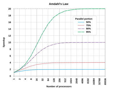
This can be seen in this graph - as you add more processors, the speedup factor stops improving.
What affects different performance metrics
| IC | CPI | T_c | |
|---|---|---|---|
| Algorithm | Y | Y | N |
| Language | Y | Y | N |
| Compiler | Y | Y | N |
| ISA | Y | Y | Y |
MIPS
In order to fully understand computer architecture, we must first understand MIPS. MIPS is an instruction set with simple instructions, which enables pipelining and parallelism. It is a RISC architecture.
Each instruction in MIPS is 4 bytes (32 bits), or a WORD of memory. They are encoded in binary, with a small number of formats. Most instructions are highly regular.
MIPS Instriction Formats
R-Format Instructions - Used for airthmetic/logical operands
| op   | rs  | rt  | rd  |shift| funct|
  6       5     5     5     5     6
I-Format Instructions - provides an immediate/constant, also used for load/store instructions
| op   | rs  | rt  |  constant/address|
  6       5     5          16
J-Foramt Instructions - provides a larger constant, used for jump instructions
| op   |         constant/address     |
  6               26
MIPS Operations
Immediate Operations - These operate on a register as well as data incoded in the instruction itself.
addi $s0, $s0, 4  //example addition, takes the value of $s0 and adds 4
addi $s0, $s9, -1 //for subtraction, just add a negative constant
This has the advantage of making common operations fast. The constant can only be 16 bits long - an appropriate trade off because small constants are the most common.
Register Operations - In MIPS arithmetic uses register operands as you can’t add two values stored in memory. In MIPS, we use a 32x32bit register file. That is we have 32 registers, each of which is 32 bits on. This is directly from our R/I-format, each register is encoded by 5 bits, so in total 32 registers are able to be encoded.
Smaller register files tend to be faster, so increasing the register file size creates a tradeoff.
Logical Operations - These are logical operations
sll //shift left logical (fills with 0)
srl //shift right logical (fills with 0)
and, andi // logical and, andi is for anding with an immediate
or, ori // logical or
nor //logical not
Arithmetic Operations - These are used for airthmetic, usually in the format a gets b + c
add $rs $rt $rd //add with register operands
addi $rs $rd 0x32 //immediate add
sub $rs $rt $rd //sub with register operands
subi $rs $rd 0x32 //immediate subtract
Conditional Operations - These are used to alter the PC
beq $rs $rt L1 // if rs==rt branch to L1
bne $rs $rt L1 // if rs!=rt bramch to L1
j L1   // jump to L1 unconditionally
Memory Operations - We need explicit instructions for memory mamagement because this is a RISC architecture.
lw $t0, 32($s3) // loads a value into memory
sw
We assume that memory is a giant array of byte-addressable words and words are aligned in memory.
Branch Operations - Used to alter the PC to control execution flow. One thing to note is that less than is slower than equivalence Create combinations of branches/subtractions as a compromise
blt
bge
slt, slti
slta, sltai
We can use branch operations to handle procedure calls.
- Place parameters in registers
- Transfer control to procedure (Change the PC)
- Acquire storage for the procedure
- Run Procedure
- Place result into a register
- Return to place of call and continue execution
jal LabelFuncStart //this changes the PC, saves the previous PC in $ra
jr $ra //jumps the PC back to where it would have been
We can see by altering $ra we alter the location of the PC, which lets us do calculated jumps as you would see in a case/switch statement.
Large Constants - Since the immediate values must fit within 16 bits, when we deal with large constants we have to store them into a register.
lui $s0 61 //load the upper 16 bits of the register
ori $s0 $s0 2304 //load the lower 16 bits
Addressing
Since memory is byte-addressable, we can omit the last 2 bits when storing an address (It’ll always be 00).
- Immediate -
- Register - Store address inside a register file and access it that way
- PC-relative - PC + offsetx4, where the x4 comes from efficient storing of bits
- Base -
- Pseudo-direct - used for J-type instructions. Takes the upper 4 bits from the current PC and concatenates the next 28 bits
Arithmetic and the ALU
One Bit Full Adder - the layout of a full adder for 1-bit operands.
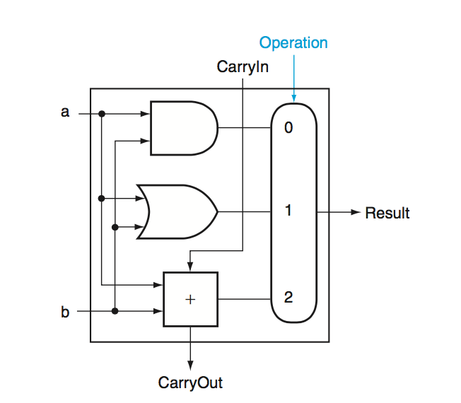
Input: ALU op, a, b, less Output: Zero, Result, Overflow, Carry Out
ALU Operations
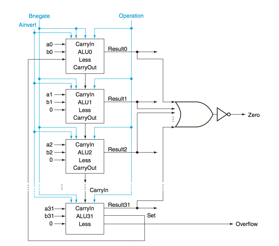
Overflow - Overflow is detected by xoring \(C_{31}\) and \(C_{32}\). When the two carry bits are different, an overflow has occured.
Zero - A single NOR gate over the results provides us with the zero output.
Addition - this can be handled by setting the mux to be the output of the full adder. The output we get out is sum of the two operands.
Subtraction - To do subtraction, we can simply negate the second operand \(b\) and add. Since we use 2’s complement encoding, this correspondings to \(-(b+1)\). To get rid of this extra \(-1\) constant we can set the initial \(C_0\) to be 1.
SLT - This is a bit tricky. We can’t do this with our existing diagram, but we can if we add a \(\textbf{less}\) input that just feeds directly through the mux. If we do this, we can do a subtraction and then link \(Result_{31}\) to \(\textbf{less}_0\), while keeping all other \(\textbf{less}\) inputs to 0 to get the desired output.
Multiplication - We can do long-multiplication in binary.
for i in range(0, 32):
  Take LSB of Multiplier
  if 1:
    Add multiplicand to product and put into the product register
  shift multiplicand left
  shift multiplier right
With this approach, if we want to multiply negative numbers. we must first invert them and then invert back accordingly.
We can also use Booth’s Algorithm, which also offers some potential speedup as well by replacing a sequence of additions with a single addition and them subtraction.
ALU Design
Ripple Carry Adder - To get a 32 bit adder, we can chain together 32 one-bit adders, connecting the output of one adder to the carry in of the one below it.
 Here we have a \(2N\) gate delay where \(N\) is the number of bits as there are 2 gates per carry out. (1 OR and 1 AND as seen from the 1-bit full adder aboce)
Carry Lookahead Adder - In order to reduce the gate delay, we can use a carry lookahead adder.
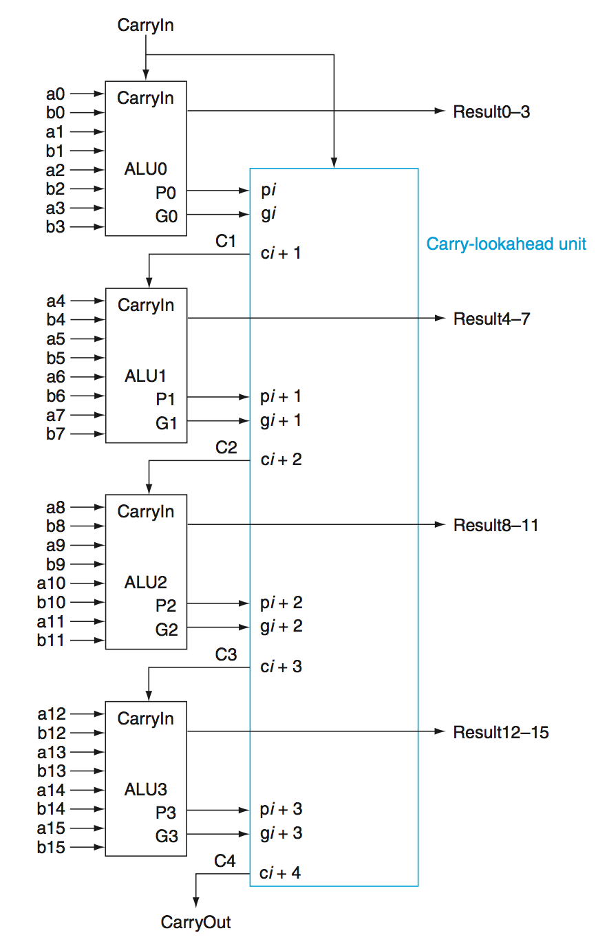
The idea here is that instead of one giant 32-bit ALU, we use multipe smaller ALUs, In this case, we don’t have to chain together the carries, we can instead compute them as a function of propogates and generates.
| A | B | Carry Out | signal |
|---|---|---|---|
| 0 | 0 | 0 | kill |
| 0 | 1 | Carry In | propagate |
| 1 | 0 | Carry In | propagate |
| 1 | 1 | 1 | generate |
As seen from the truth table, propogates can be represented by an OR gate, while generates can be represented as an AND gate.
\[C_1 = G_0 + C_0P_0\] \[C_2 = G_1 + G_0P_1 + C_0P_0P_1\] \[C_3 = G_2 + G_1P_2 + G_0P_1P_2 + C_0P_0P_1P_2\] \[C_4 = G_3 + G_2P_3 + G_1P_2P_3 + G_0P_1P_2P_3 + C_0P_0P_1P_2P_3\]This creates a larger but faster adder.
Carry Select Adder - This is simply two adders, one for a potential carry of 1 and one for a 0 carry, We run the computation on both adders and use a mux to select the results. This gives us much better performance but at the expense of a much larger adder.
Single Cycle Processor
We start by considering a simple subset of operations -
lw, sw, add, sub, and, or, slt, beq, j
The processor cycle can be descripbed as a continuous loop between 5 stages:
- Instruction Fetch (IF)
- Instruction Decode (ID)
- Execute (EX)
- Acces Memory (MEM)
- Store Result (WB)
Instruction Execution - we grab the instruction at the location in program memory via the PC
Pipelining
In order to improve performance, we can overlap execution of instructions to reach a steady state, where CPI reaches it’s asymptotic mininum.
If all stages are balanced, then \(T_{pipeline} = \frac{T_{sequential}}{n}\) where \(n\) is the number of stages. Otherwise, \(T_{pipeline} = \max(T_i)\) where \(T_i\) is the time taken for each part of the pipeline.
MIPS is well suited for pipelining - all instructions are 32-bits, and are very regular. Furthermore, memory access only takes 1 cycle.
In order to pipeline properly, we must uphold several principles.
- Must have same stages in the same order
- All intermediate values must be latched
- We cannot use the same functional block twice in a single cycle
Pipelining also introduces hazards into the pipeline, where the pipeline must stall and performance drops.
Hazards
Data Hazards - need to wait for previous instruction to complete to get the correct data.
add $3, $10, $11
lw $8, 50($3)
sub $11, $8, $7
Either insert independent instruction/no-ops as a software fix or stall the pipeline/employ data-forwarding as a hardware fix. One thing to note is that the software fix ruins the portability of the application.
We can try to miniimze stalls by restructuring the instruction layout via some sort of topological sort.
Structural Hazards - Occur when two instructions want to use the same resource. For example consider a LW and a SW, they would both try to use the IF instruction stage at the same time. Hence pipelined datapaths require seprate instruction/data memory.
Control Hazards - Deciding on control action depends on a previous instruction.
There are two main types of control hazards -
Instruction Level Parallelism
In order to run faster, we need to exploit more parallelism. Ideally, we could execute multiple instructions in parallel. One way we can do this is via multiple issue.
Multiple Issue
Multiple issue can be broken down to static multiple issue (VLIW) where the compiler groups independent instructions together into issue slots and dynamic multiple issue where the CPU examines the instruction stream and resolves hazards at runtime.
static multiple issue has the advantage of being much simpler, at the expense of portability. Generally, there is a slot for Branch/ALU instructions and a slot for Load/Store instructions.
Dependencies within packets are not allowed but between packes its fine. However there are several changes that we have to make before multiple issue will work.
Firstly, we need to expand the register file to output more than 2 registers, then add another ALU/adder.
Next we need to modify the PC to shift 8 bytes instead of 4.
We will of course run into hazards - nalmely we can’t use the ALU result in the same packet and there is no forwarding between two instructions in a packet. The Load-Use data hazard also effectivley doubles, as stalling once represents missing out of the execution of two instructions. As a result, we try to use more aggressive compilers and schedulers when we use multiple issue.
One example of this is loop unrolling, where we can unroll a loop so that it can be executed faster.
In dynamic multiple issue the CPU will execute instructions out of order but then commit results in order. For this to work we need register renaming.
Memory and Caching
We treat memory as a large quickly-accessible byte-addressable array, but in reality no memory has these characteristics. As a result, we must exploit locality. There are two types of locality, spatial locality and temporal locality
spatial locality refers to the tendency of us to visit the locations adjacent to our target.
temporal locality refers to the tendency of us to visit a location we previously already visited.
By using caches to exploiting temporal and spatial locality we can make memory look like a large, quickly-accessible byte-addressed array, when in fact it is not.
Associative Caches
Caches have different levels of associativity. A fully associative cache is one where any element can go to any slot of the cache. This is sort of like a hash table with a fixed number of buckets.
Increasing the block size makes a cache more able to exploit spatial locality but will increase the number of misses.
On cache misses we must stall the pipeline until the result is returned. However there are different ways in which we can deal with cache misses.
- write-through - On a cache miss, we first write our changes to the cache, and then write our changes to memory.
- write-back - On a cache miss, we write our changes to the cache, and then set a dirty bit. When that cache block is removed, we check if the dirty bit is set - if it is we write all changes to memory.
- write-allocate - On a cache miss we bring that block of memory into the cache.
- write-arround - On a cache miss we don’t bring that block of memory into the cache, but rather just write our changes directly into memory.
We can categorize cache misses into three types
- compulsary - These are cache misses that occur because the cache is not yet filled.
- capacity - Occurs when all the slots in the cache are filled.
- conflict - Occurs when there is room in the cache, but the cache block that we specifically want to fill is occupied
Multi-level cahces, Virtual memory and page faults (TLB)
VIPT vs VIVT vs PIPT Cache coherence, snooping and snarfing,